Bifurcating Lease Embedded FX Derivatives

Section I.  Overview

Suppose an entity enters into an agreement to lease property and make rental payments each month, but that the fixed notional underlying the lease payments is denominated in some other currency.  This introduces an exposure for the lessee (but not for the lessor) since now they must pay a domestic currency equivalent of some fixed amount in a foreign currency - in other words, they pay Lease Payment x Exchange Rate, whatever that might be at the time the payment becomes due.  If the entity is a corporate entity, accounting regulations require the entity to "bifurcate" the embedded derivative from the contract and account for it as though it was a legitimate derivative, per the rules of derivative accounting.  This introduces accounting complexities, but the problem must also of course be solved from a valuation point of view.


In this post we consider lease agreements as just described, as well as those with caps and floors on the exchange rate with strikes contractually written into the agreements.


Section II.  Valuation Methodology


For leases determined to have embedded derivatives (from the point of view of the domestic entity), we value the embedded derivative as a strip of component derivatives corresponding to each future cash flow. That is, each cash flow represents the notional (denominated in the foreign currency CUR1) for each component derivative, and value of the lease embedded derivative is the aggregate value of these component derivatives.

Our FX convention is CUR1/CUR2 where this rate is the \# units of CUR2 per 1 unit of CUR1 - such a quantity has units [CUR2]/[CUR1]. We refer to CUR2 as the domestic, functional and settlement currency and CUR1 as the foreign, deal and notional currency.

Our valuation methodology is based on usual market-practice - in particular, no arbitrage and discounted cash flow principles. For options, we use the additional assumption of no-arbitrage for an asset price following a simple geometric Brownian motion (Black-Scholes-Merton model). Consider a present valuation date $t$, future maturity date $T>t$, future cash flow $N=N(T)$, corresponding strike rate $K=K(T)$, forward rate $F=F_{t}(T)$, discount rate $D=D_{t}(T)$ and volatility $\sigma=\sigma_{t}(K,T)$. Let $V=V_{t}(T,N,K,F,D,\sigma)$ denote the value of a derivative written on CUR1/CUR2 with the previous parameters. Then our previous assumptions lead us to the following valuation formulas: $$(1)\;\;\;\;V^{\text{fwd}}_{t}(T)=N(T)\cdot(F_{t}(T)-K(T))\cdot D_{t}(T)$$
$$(2)\;\;\;\;V^{\text{call}}_{t}(\Phi(d_{+})F_{t}(T)-\Phi(d_{-})K)\cdot D_{t}(T),$$
and
$$(3)\;\;\;\;V^{\text{put}}_{t}(T)=(\Phi(-d_{-})K-N(-d_{+})F_{t}(T))\cdot D_{t}(T).$$
In (2) and (3) we define
$$d_{\pm}=\frac{1}{\sigma_{t}(K,T)\sqrt{T-t}}\left[\log\left(\frac{F_{t}(T)}{K(T)}\right)\pm\frac{1}{2}\sigma_{t}(K,T)^{2}(T-t)\right]$$
and
$$\Phi(x)=(2\pi)^{-1/2}\int_{-\infty}^{x}e^{-y^{2}}{2}\;dy,$$
the standard normal cumulative distribution function.
(Note the dependence of $\sigma_{t}$ on $(K,T)$ is due to the nature of FX option markets exhibiting term structure variation and ``smiles.'')

Section III.  Extraction Methodology

Section III(a).  Specifying the Strike

We extract the embedded derivative in accordance to the principle that the stated value of the cash flow at inception of the lease agreement should be such that the value of the embedded derivative at inception is $0$. We appy this principle to the forward component of the embedded derivative, and approximate it by assuming the cancellation between the cap and floor values (because one is a short position and the other is a long position - see below) would net $0$ if we assumed that they constitute a forward in combination. This is exactly true from put-call parity when the strikes are the same, but only approximately true if they are different (which they must be since otherwise the combination of the three instruments would net $0$ and there would be no embedded derivative). In particular, if the lease agreement has $i=1,2,3,\ldots,n$ future cash flows, a cap $\overline{S}=\overline{S}(T_{i})$ and a floor $\underline{S}=\underline{S}(T_{i})$, then for each corresponding component derivative we set (where again, $t=0$ is the inception date of the lease): $$(4)\;\;\;\;K^{\text{fwd}}(T_{i})=F_{0}(T_{i}),$$ $$(4)\;\;\;\;K^{\text{cap}}(T_{i})=\overline{S}(T_{i}),$$ and $$(4)\;\;\;\;K^{\text{flr}}(T_{i})=\underline{S}(T_{i}).$$ Accounting rules indicate that this is the proper approach from a valuation point of view.

Section III(b).  Specifying the Derivative - A Decomposition

In keeping with our notation, we let $L_{t}(T_{i})$ denote the present fair value at time $t$ of the future cash flow made at time $T_{i}$. This is always a negative quantity from the entity's point of view. The idea in order to obtain the embedded derivative is to separate the risky portion of this value from the non-risky portion. In particular, we decompose $L_{t}(T_{i})$ as
$$L_{t}(T_{i})=B_{t}(T_{i})+Z_{t}(T_{i}),$$
where $B_{t}(T_{i})$ only depends on $t$ through the discounting at time $t$ $D_{t}(T_{i})$ (in particular, it is independent of market variables like $F_{t}(T_{i})$), and $Z_{t}(T_{i})$ is a function of all random market variables inherent in $L_{t}(T_{i})$. There are an infinite number of ways to structure such a decomposition, but accounting guidance discussed above is equivalent to certain initial and terminal conditions which allow us to uniquely solve for $B(T_{i})$ and $Z(T_{i})$.

Section III(c).  Specifying the Derivative - Forward Only Case

If the lease payment $L_{t}(T_{i})$ lacks any optional features, then its payoff is
$$L_{T_{i}}(T_{i})=-N\cdot S_{T_{i}}$$
and therefore its fair present value for $0<t<T_{i}$ is given by $$(7)\;\;\;\;L_{t}(T_{i})=-N(T_{i})\cdot F_{t}(T_{i})\cdot D_{t}(T_{i}).$$ Observe that this quantity has units of CUR2 and this is the present value of what the entity has to pay at time $T_{i}$. Since it depends on the forward rate $F_{t}(T_{i})$, it has an exposure to CUR1/CUR2 and is therefore risky. The ideas previous discussed involves decomposing $L_{t}(T_{i})$ into two parts $$L_{t}(T_{i})=B_{t}(T_{i})+Z_{t}(T_{i}),$$ where $B_{t}(T_{i})$ only depends on $t$ through $D_{t}(T_{i})$ (in particular, it is independent of $F_{t}(T_{i})$), and $Z_{t}(T_{i})$ is a function of $F_{t}(T_{i}).$ The initial condition $$Z_{0}(T_{i})=0$$
and
terminal payoff condition
$$L_{T_{i}}(T_{i})=B_{T_{i}}(T_{i})+Z_{T_{i}}(T_{i})=N(T_{i})\cdot F_{T_{i}}(T_{i})\cdot D_{T_{i}}(T_{i})=-N(T_{i})\cdot S_{T_{i}}$$
allow us to uniquely solve for the payoff of $B(T_{i})$ and $Z(T_{i})$, the principle of rational pricing and the fact that $B_{t}(T_{i})$ is a constant in $t$ (ignoring discounting) then gives us $L$, $B$, and $Z$ for all $0<t<T_{i})$. Indeed, from the terminal condition we have
$$Z_{T_{i}}(T_{i})=-N(T_{i})\cdot S_{T_{i}}-B_{T_{i}}(T_{i})$$
and from the initial condition
$$B_{0}(T_{i})=L_{0}(T_{i})=-N(T_{i})\cdot F_{0}(T_{i})\cdot D_{0}(T_{i})=-N(T_{i})\cdot K^{\text{fwd}}(T_{i})\cdot D_{0}(T_{i}).$$
Hence (dropping the ``fwd'' from $K$),
$$Z_{T_{i}}(T_{i})=-N(T_{i})\cdot(K(T_{i})-S_{T_{i}}).$$
This shows that the payoff of $Z(T_{i})$ is equal to a short position in CUR1/CUR2 with notion $N(T_{i})$. Applying our reasoning above, we discover $Z_{t}(T_{i})$ is given by (2). Explicitly,
$$(8)\;\;\;\;Z_{t}(T_{i})=-N(T_{i})\cdot(K(T_{i})-F_{t}(T_{i}))\cdot D_{t}(T_{i})$$br /> and
$$(9)\;\;\;\;B_{t}(T_{i})=-N(T_{i})\cdot K(T_{i}).$$

Section III(c).  Specifying the Derivative - Ranged Forward Case (Caps & Floors)

If $L_{t}(T_{i})$ has optional features, then the initial condition $Z_{0}(T_{i})$ is replaced by the value of these optional features using the strike prices given by (5) and (6). For a ranged forward, we have a cap $\overline{S}(T_{i})$ and a floor $\underline{S}(T_{i})$. With our FX convention CUR1/CUR2, the terms ``cap'' and ``floor' are really as such from the counter-party's perspective, or from the entity's perspective when considering the value of the overall lease $L_{t}(T_{i})$ (a cap and floor on how much the entity has to pay). However, when considering the value of $Z_{t}(T_{i})$ from the entity's, the cap $\overline{S}(T_{i})$ is an upper-bound on how much CUR2 can weaken against CUR1, hence a floor ($=1/\overline{S}(T_{i})$) on their losses from their short position in the forward component of the embedded derivative. Conversely, the floor $\underline{S}(T_{i})$ is a lower-bound on how much CUR2 can strengthen against CUR1 hence a cap ($=1/\underline{S}(T_{i})$) on their gains.

The previous paragraph shows that $Z_{t}(T_{i})$ is a sum the sum of three distinct derivatives $\sum_{k=1}^{3}Z^{k}_{t}(T_{i})$ - a short position in a put option on CUR1/CUR2 struck at $\underline{S}(T_{i})$, a long position in a call option on CUR1/CUR2 struck at $\overline{S}(T_{i})$, and a short position in a forward on CUR1/CUR2 struck at $K(T_{i})=F_{0}(T_{i}).$ This can be proved as we did for the case of a forward, where the initial condition is taken to be $$Z_{0}(T_{i})=\sum_{k=1}^{3}Z^{k}_{0}(T_{i})=V^{\text{call}}_{0}(T_{i})-V^{\text{put}}_{0}(T_{i})+\underbrace{V^{\text{fwd}}_{0}(T_{i})}_{=0},$$
as given by (1), (2) and (3), respectively.
The terminal condition is
$$L_{T_{i}}(T_{i})=\left\{\begin{array}{ll}-N(T_{i})\cdot\overline{S}(T_{i}),&S_{T_{i}}>\overline{S}(T_{i})\\-N(T_{i})\cdot S_{T_{i}},&\underline{S}(T_{i})\leq S_{T_{i}}\leq\overline{S}(T_{i})\\-N(T_{i})\cdot \underline{S}(T_{i}),&S_{T_{i}}<\underline{S}(T_{i}).\end{array}\right.$$
It follows that
$$B_{0}(T_{i})=-N(T_{i})\cdot K(T_{i})\cdot D_{0}(T_{i})$$
and hence
$$B_{t}(T_{i})=-N(T_{i})\cdot K(T_{i})\cdot D_{t}(T_{i})$$
for all $0<t<T_{i}.$ Now,
$$Z_{T_{i}}(T_{i})=L_{T_{i}}(T_{i})-B_{T_{i}}(T_{i})=\left\{\begin{array}{ll}K(T_{i})-\overline{S}(T_{i}),&S_{T_{i}}>\overline{S}(T_{i})\\K(T_{i})-S_{T_{i}},&\underline{S}(T_{i})\leq S_{T_{i}}\leq\overline{S}(T_{i})\\K(T_{i})-\underline{S}(T_{i}),&S_{T_{i}}<\underline{S}(T_{i}).\end{array}\right.$$
One verifies easily that this is equal to
$$Z_{T_{i}}(T_{i})=-(S_{T_{i}}K(T_{i}))+\max(S_{T_{i}}-\overline{S}(T_{i}),0)-\max(\underline{S}(T_{i})-S_{T_{i}},0)$$
which are the payoff functions of the indicated derivatives. Thus,
$$(10)\;\;\;\;Z_{t}(T_{i})=-A+B-C$$
for all $0<t<T_{i}$ where $A$ is given by (1), $B$ by (2) and $C$ by (3).


Section IV Lease Modifications - An Introduction

In a subsequent post I will elaborate on the bifurcation and valuation of modifications to lease agreements.  For now, let us keep in mind the above consider a typical lease cash flow $L_{t}(T)$ with a notional of $N$.  At the time the lease is entered into, FASB requires bifurcation of any implied derivative $Z$. Suppose $Z$ is just an FX forward (short CUR1/CUR2).  At inception ($t=0$) the strike is $K_{0}=F_{0}(T)$, the forward rate corresponding to the future time $T$ as calculated at time $t=0$. The value of $Z$ at any time $0<t<T$ is
$$Z_{t}(N_{0},K_{0},T)=N_{0}\cdot(K_{0}-\cdot F{t}(T))\cdot D_{t}(T),$$
where $D_{t}(T)$ is the discount factor for term $T$ at time $t$. This valuation methodology makes the embedded derivative $0$ at inception of the lease.

Suppose at some time $0<\tau<T$ we have the modification $N_{0}\mapsto N_{\tau}<N_{0}$ (the lease payment decreases). Then this is economically equivalent to maintaining the unmodified lease and entering into another lease with notional $\Delta N_{0,\tau}:=N_{0}-N_{\tau}$ as a lessor at the time of modification $\tau$. FASB would then require the lessor to put the resulting embedded derivative on their balance sheet that time.  The value of this derivative (since it is equivalent to a long position in CUR1/CUR2 or short CUR2/CUR1) is
$$\tilde{Z_{t}}(\Delta N_{0,\tau},K_{\tau},T)=\Delta N_{0,\tau}\cdot(F_{t}(T)-K_{\tau})\cdot D_{t}(T).$$
Now, from an operational lease accounting point of view, the P/L at the cash flow date is just $N_{0}-\Delta N_{0,\tau}=N_{\tau}.$ Therefore, the net embedded derivative of this overall lease contract is $Z+\tilde{Z}$ (the ``+'' is actually a ``-'' since we modeled $\tilde{Z}$ as a long position). Thus, the derivative's value at all times $\tau<t<T$ is
$$\begin{align*}
Z^{\tau}_{t}(N_{\tau},K_{\tau},T)
&=Z_{t}(N_{0},K_{0},T)+\tilde{Z_{t}}(\Delta N_{0,\tau},K_{\tau},T)\\
&=N_{0}\cdot(K_{0}-F_{t}(T))\cdot D_{t}(T)+\Delta N_{0,\tau}\cdot(F_{t}(T)-K_{\tau})\cdot D_{t}(T)\\
&=D_{t}(T)\Big[N_{0}K_{0}-N_{0}F_{t}(T)+N_{0}F_{t}(T)-N_{0}K_{\tau}-N_{\tau}F_{t}(T)+N_{\tau}K_{\tau}\Big]\\
&=N_{0}\cdot(K_{0}-K_{\tau})\cdot D_{t}(T)+N_{\tau}\cdot(K_{\tau}-F_{t}(T))\cdot D_{t}(T)\\
&=N_{0}\Delta K_{0,\tau}D_{t}(T)+N_{\tau}\cdot(K_{\tau}-F_{t}(T))\cdot D_{t}(T)\\
&=N_{\tau}(K_{\tau}-F_{t}(T))\cdot D_{t}(T)+C
\end{align*}$$
where the constant $C$ is the settlement price at time $T$ made at time $\tau$ and discounted to time $\tau<t<T$.

Can a Derivative's Value Exceed the Underlying Notional Value?

On a recent project I valued some derivatives, the results of which the client balked at because the values exceeded the notional on which they were written.  So is it ever possible for a derivative's valuation to exceed its underlying notional?


The answer, of course, depends, and first we need to clarify what we mean by a derivative's value exceeding its notional.  A typical derivative (like an option or future) is written on some underlying asset with price $S_{t}$ and some quantity or notional $N$.  The term quantity is frequently used for assets like stocks and the term notional for assets like currencies - so in the latter case, if I have USD/EUR call option, then I view the asset as the US dollar (that I want to buy a call option on) priced in the European Euro (that is what the USD/EUR exchange rate is - the cost of a US dollar in Euros), with a notional (i.e. quantity) equal to (say) $\$100,000,000$ USD.

Notice that the quantity/notional has units in the underlying asset and that the spot price $S_{t}$ has units of value in the numeraire/settlement currency per 1 asset.  Hence, when we ask if a derivative's value can exceed its underlying notional, we are really asking whether the value at time $t$, denoted $V_{t}$, can exceed the quantity $NS_{t}$, which has units in the settlement currency (EUR in the above example).  In other words, we ask whether
$$V_{t}>NS_{t}$$
can hold without introducing an arbitrage.

Essentially, the purpose of the above discussion was to express precisely what we mean for the valuation to exceed the underlying notional and moreover, to emphasize that derivative's valuation cannot be directly compared to the notional in order to answer the question, since since the units are not the same - the underlying notional $N$ needs to be multiplied by the spot price $S_{t}$ so that each has units in the valuation currency.

The classic counter-example to answering this question affirmatively in all instances comes from considering a call on option written on $N$ of some asset with price $S_{t}$.  If you value this option at time $t$, then it is clear that
$$V_{t}<NS_{t},$$
for otherwise one could short a covered option at no cost and an arbitrage would exist.  But this argument no longer holds for instruments with payoffs that are not artificially bounded by some optionality mechanism.  Indeed, the example from my experience involved an FX forward on CUR1/CUR2 (to be generic).  For such a forward, let $K$ be the strike, $N$ the notional (denominated in CUR1), $D$ the discount factor and $\alpha$ the CUR2/CUR1 exchange rate ($1/S_{t}$).  Then if the entity is in the short position we have
$$-\alpha N\cdot(F-K)\cdot D>N$$
$$(F-K)<-\frac{1}{\alpha D}$$
$$F<K-\frac{1}{\alpha D}.$$
Hence, if the forward rate is sufficiently small (i.e. price of CUR1 declined) with respect to the inception strike, then the value of the forward will exceed the notional as an asset. Conversely,
$$-\alpha N\cdot(F-K)\cdot D<-N$$
$$(F-K)>\frac{1}{\alpha D}$$
$$F>K+\frac{1}{\alpha D}$$
Hence, if the forward rate is sufficiently large (i.e. the price of CUR1 increased) with respect to the inception strike, then the value of the forward will exceed the notional as a liability.

It is not difficult to come up with similar bounds for other basic instruments such as swaps either.

A Simple Monte Carlo Simulator for European Call Options

In this post I will present a procedural C++ implementation of a simple Monte Carlo simulator for the pricing of a European call option.  Subsequent articles will make significant improvements such as the pricing of puts and different types of options, improved sampling, incorporation of jump processes, etc.

Recall that we model a stock price $S$ as a stochastic process $\{S_{t}:0\leq t\leq T\}$ governed by the stochastic differential equation (geometric Brownian motion)
$$(1)\;\;\;\;dS_{t}=\mu S_{t}dt+\sigma S_{t}dW_{t}$$
where $\mu$ is the drift or expected return on the stock, $W_{t}$ is a Weiner process $(dW_{t}=N(0,1)\sqrt{dt}$ where $N(0,1)$ is the standard normal distribution), and $\sigma$ is the volatility of the stock (a measure of the variance since $\sigma N(0,1)=N(\sigma^{2},1)$).  Using arbitrage arguments (Merton's method) we arrive at the (linear) Black-Scholes-Merton partial differential equation
$$(2)\;\;\;\;V_{t}+\frac{1}{2}\sigma^{2}S^{2}V_{ss}+rSV_{s}-rV=0.$$ The price $V$ of any derivative must satisfy this equation, and conversely, any solution to (2) gives the price of some derivative based on the boundary conditions used (for European call options, the boundary conditions at the expiry time $T$ are $V(\cdot,T)=\max(S_{T}-K,0)$ where $K$ is the strike price of the option and $S_{T}$ is the value of the (random) stock price at time $T$).  Pricing methods for derivatives based on (2) are known as PDE methods in mathematical finance, and usually consist of numerically solving (2) using finite difference methods (since the domain of definition is rectangular in the $(S,t)$ coordinate system).  This can be difficult, however, since the varied boundary conditions must be taken into account and issues of convergence, stability, etc. enter in.

A different (and more recently popular) approach is probabilistic and involves sampling the randomness in the geometric Brownian motion model (1) of the stock price multiple times and taking an average.  Indeed, an application of the Feynman-Kac formula shows that when discounted appropriately, solutions to (1) are martingales and this implies that $V$ is simply the expected value of the discounted payoff of the derivative.  For a European call option, the payoff is $f(S)=\max(S-K,0)$ and so we get
$$(3)\;\;\;\;V_{\text{EuroCall}}=e^{-rT}\mathcal{E}[f(S_{T})]$$
where $r$ is the riskless return, $\mathcal{E}$ is taken under the risk-neutral probability measure, and $S_{T}$ is the final value of the stochastic process $\{S_{t}\}$ at expiry of the option $T$.  (From now on, $V$ is for the price of a European call option.)  Thus, beginning with (1), passing to the logarithm, applying Ito's Lemma and then applying (3) we get
$$\begin{align*}
&dS_{t}=rS_{t}\;dt+\sigma S_{t}dW_{t}\\
\Longrightarrow&d\log S_{t}=(r-\frac{1}{2}\sigma^{2})dt+\sigma dW_{t}\\
\Longrightarrow&\log S_{t}=\log S_{0}+(r-\frac{1}{2}\sigma^{2})t+\sigma W_{t}\\
\Longrightarrow&S_{t}=S_{0}\exp\left\{\left(r-\frac{1}{2}\sigma^{2}\right)t+\sigma\sqrt{T}N(0,1)\right\}\\
\Longrightarrow&V=e^{-rT}\mathcal{E}\left[f\left(S_{0}\exp\left\{\left(r-\frac{1}{2}\sigma^{2}\right)t+\sigma\sqrt{T}N(0,1)\right\}\right)\right]\\
(4) \Longrightarrow&V=e^{-rT}\mathcal{E}\left[\max\left(S_{0}\exp\left\{\left(r-\frac{1}{2}\sigma^{2}\right)t+\sigma\sqrt{T}N(0,1)\right\}-K,0\right)\right]\\
\end{align*}$$

(Recall that $dW_{t}=N(0,1)\sqrt{dt}$ and so $W_{T}=N(0,1)\sqrt{T}$).  The above computations are somewhat complicated when carried out in detail, and while the explanation for how (2) is derived from (1) is relatively straight-forward, the derivation of (3) from (1) (and thus the previous computations) is significantly more subtle but far more important in the theory of mathematical finance.  A full explanation of the concepts involved (properties of Weiner processes, stochastic integration and Ito's lemma, risk-neutral valuation and the risk-neutral measure, change of numeraire, etc.) is beyond the scope of this post but will be elaborated on in subsequent posts.  In any event, we only need to take faith that (4) is equivalent to (2) for pricing European call options.

The idea of Monte Carlo simulation is now evident. We simulate $N$ paths of $S_{T}$ by sampling from the standard normal distribution $N(0,1)$ and then compute $f(S^{n}_{T})$.  Since each sampling is independent, the random variables $\{f(S_{T}^{n})\}_{n}$ are independent and identically distributed and so the law of large numbers implies
$$\frac{1}{N}\sum_{n=1}^{N}f(S^{n}_{T})\to\mathcal{E}[f(S_{T})]\;\text{as}\;N\to\infty$$
pointwise (and of course, in probability).  We then then discount at $e^{-rT}$ and this is our estimate on the price $V$.

The following implementation is coded procedurally in C++ and prices a European call option using the method explained above.  The only part which may require explanation is the method in which $N(0,1)$ is sampled.  While there are several ways to do this, a simple yet accurate/efficient method is known as the Box Muller algorithm, implemented here.

MonteCarloMethod_Source.cpp

#include <iostream>
#include <cmath>

using namespace std;

double BoxMullerGaussian();
double MonteCarloSimulator(double Expiry, double Strike, double Spot, double Vol, double Riskless, unsigned long N);

int main(void) {
 double Expiry, Strike, Spot, Vol, Riskless, N = 0;
 cout << "Enter: Expiry, Strike, Spot, Vol, Riskless, # Trials" << endl;
 cin >> Expiry >> Strike >> Spot >> Vol >> Riskless >> N;

 cout <<  "The price of the option is "
  << MonteCarloSimulator(Expiry, Strike, Spot, Vol, Riskless, N)
  << endl;
 
 double pause;
 cin >> pause;

 return 0;
}

double BoxMullerGaussian() {
 double x,y;
 
 double sizeSquared;
 do {
  x = 2.0*rand()/(double)(RAND_MAX) - 1;
  y = 2.0*rand()/(double)(RAND_MAX) - 1;
  sizeSquared = x*x + y*y;
 } while(sizeSquared >= 1.0);

 return x*sqrt(-2*log(sizeSquared)/sizeSquared);
}

double MonteCarloSimulator(double Expiry, double Strike, double Spot, double Vol, double Riskless, unsigned long N) {
 double var = Vol*Vol*Expiry;
 double std = sqrt(var);
 double itoCorrection = -0.5*var;
 double movedSpot = Spot*exp(Riskless*Expiry + itoCorrection);
 double _Spot = 0;
 double runningSum = 0;

 for (unsigned long i=0; i<N; i++) {
  double _Gaussian = GetOneGaussianByBoxMuller();
  _Spot = movedSpot*exp(std*_Gaussian);
  double _Payoff = _Spot - Strike;
  _Payoff = _Payoff>0 ? _Payoff : 0;
  runningSum += _Payoff;
 }

 return exp(-Riskless*Expiry)*(runningSum/N); // expectation
}

As an example, we consider Microsoft's stock. Today it closed at 41.35, so $\text{Spot}=41.35$ (the spot price in option pricing is $S_{0}$, which is not random, but $S_{t}$ is for $t>0$ upto $t=T=\text{Expiry}$). We write the option with a strike price $\text{Strike}=40.00$ so that the option is in the money initially (for the buyer). If the time to expiry is 6 mo., then $\text{Expiry}=0.5$. The 6mo. risk-free rate is $\text{Riskless}=0.33$ (taken to be the LIBOR rate quoted this week). The implied 6mo. volatility for Microsoft options is around $\text{Vol}=0.22$. With these parameters and $N=100$ trials, we get $$V_{\text{MSFTEuroCall}}=8.98$$

Explicit Finite Difference Method for Black-Scholes-Merton PDE (European Calls)

Here we will implement a basic finite difference method to the solution of the Black-Scholes-Merton PDE
$$(1)\;\;\;\;\frac{\partial V}{\partial t}+\frac{1}{2}\sigma^{2}S^{2}\frac{\partial^{2}V}{\partial S^{2}}+rS\frac{\partial V}{\partial S}-rV=0,$$
which of course models the value $V$ of any derivative contract in the absence of arbitrage (see the Wikipedia article for a more comprehensive list of assumptions under which the Black-Scholes-Merton model is valid).

This PDE is a backwards diffusion (parabolic) equation: it is ill-posed in forward time.  This means that "initial conditions" are prescribed at $t=T$, the expiry time of the derivative being priced (in the case of this article, an option).  This is analogous to the prototypical heat equation $u_{t}=\Delta u,$ which is ill-posed in backward time, and hence requires initial conditions to be prescribed at time $t=0$.  It makes sense that a reverse-time evolution equation would model the value of a derivative since the payoff of the conract is known at the time of expiry $t=T$, and it is at the initial time $t=0$ that we are interested in knowing the "correct" value of the contract.  Indeed, we assume that the underlying of the derivative is a stock which follows a geometric Browning motion $\{S_{t}\}_{t\geq0}$ as in the Black-Scholes-Merton model.  This is a stochastic process for which we know $S_{0}$ (the time that the contract is being sold) and so the Black-Scholes equation allows us to compute $V(S(t),t)\big|_{t=0}=V(S_{0},0)$, which is the value of the contract today with observed stock price $S_{0}$.

The above discussion gives us an indication as to what boundary conditions must be prescribed in order that the solution $V(S,t)$ corresponds to the particular derivative contract being valued.  Indeed, (1) gives the value of any derivative; it is the boundary conditions which specify which derivative.  We shall consider the PDE to be defined on the $(S,t)$ space $[0,\bar{S}]\times[0,T]$ where $\bar{S}$ is the maximal stock price (typically $\bar{S}$ is taken to be $\bar{S}\approx 3K$, where $K$ is the strike price of the option).  (Ideally, we would have $\bar{S}=\infty$ so that we could apply the natural bounary condition $V(S,t)\to S$ as $S\to\infty$, but we must use a finite domain when applying finite differences.)  We then have the following boundary-value problem corresponding to (1)

$$\left\{\begin{array}{ll}
\frac{\partial V}{\partial t}+\frac{1}{2}\sigma^{2}S^{2}\frac{\partial^{2}V}{\partial S^{2}}+rS\frac{\partial V}{\partial S}-rV=0,&0\leq t< T, 0<S<\bar{S}\\
V(S,T)=\max(S-K,0),&t=T\\
V(0,t)=0,&S=0\\
V(\bar{S},t)=\bar{S}-Ke^{-r(T-t)},&S=\bar{S}.\end{array}\right.
$$

We now discretize the domain into increments $\Delta S$ and $\Delta t$.  The following notation is used: $k=\Delta t$, $h=\Delta S,$ $V_{m}^{n}=V(mh, nk),$ $N=T/k$, $M=\bar{S}/h.$  For simplicity we start with forward differences in time and centered differences in space to get (after some algebra)
$$V_{m}^{n}=A_{m}V_{m-1}^{n+1}+B_{m}V_{m}^{n+1}+C_{m}V_{m+1}^{n+1}$$
where
$$\begin{array}{l}
A_{m}=\frac{k}{2}\left(\sigma^{2}m^{2}-rm\right)\\
B_{m}=(1-k)(r\sigma^{2}m^{2})\\
C_{m}=\frac{k}{2}\left(\sigma^{2}m^{2}+rm\right)\end{array}
$$

Recall that the evolution is backward in time, so that this method is indeed explicit.

The following method was coded in Excel VBA using the method discussed above.  In this implementation we have used parameters $T=0.25$ (expiry in 3 months), $K=10$ (strike price 10 USD), $r=0.1$ and $\sigma=0.4.$

BS_FDM_Explicit.xlsm (Coded in Excel VBA)

Sub BSFiniteDifferenceScheme()

    ' User defined parameters
    Dim Riskless As Double
    Dim Vol As Double
    Dim Expiry As Double
    Dim Strike As Double
    
    Riskless = 0.1
    Vol = 0.4
    Expiry = 0.25
    Strike = 10
    
    ' Finite difference parameters
    Dim T As Double ' final time
    Dim S As Double ' stock price upper limit
    Dim N As Integer ' temporal steps
    Dim M As Integer ' stock steps
    Dim k As Double ' time step
    Dim h As Double ' stock step
    Dim V() As Double ' solution V(s,t)
    Dim T_Array() As Double
    Dim S_Array() As Double
    
    ' Set preliminary parameters
    T = Expiry
    S = 30
    k = 0.001
    h = 0.5
    N = T / k
    M = S / h
    ReDim V(N, M)
    
    For i = N To 0 Step -1
        Cells(i + 2, 1) = i * k
    Next i
    For j = 0 To M
        Cells(1, j + 2) = j * h
    Next j
    
    ' Set left boundary condition (S=0)
    For i = N To 0 Step -1
        V(i, 0) = 0
        Cells(i + 2, 2) = V(i, 0)
    Next i
    
    ' Set upper boundary condition (t=T)
    For j = 0 To M
        If j * h > Strike Then
            V(N, j) = j * h - Strike
        Else
            V(N, j) = 0
        End If
        Cells(N + 2, j + 2) = V(N, j)
    Next j
    
    ' Set right boundary condition (S=S_max)
    For i = N To 0 Step -1
        V(i, M) = S - Strike * Exp(-Riskless * (T - i * k))
        'V(i, M) = S
        Cells(i + 2, M + 2) = V(i, M)
    Next i
    
    ' Computation Loop
    Dim A As Double
    Dim B As Double
    Dim C As Double
    For i = N - 1 To 0 Step -1
        For j = 1 To M - 1
            A = (k / 2) * (Vol ^ 2 * j ^ 2 - Riskless * j)
            B = 1 - k * (Riskless + Vol ^ 2 * j ^ 2)
            C = (k / 2) * (Vol ^ 2 * j ^ 2 + Riskless * j)
            V(i, j) = A * V(i + 1, j - 1) + B * V(i + 1, j) + C * V(i + 1, j + 1)
            Cells(i + 2, j + 2) = V(i, j)
        Next j
    Next i
   
End Sub

The output has been setup to give the value of $V(S,t)$ for any pair $(S,t)$.  The table of data is of course to large to be given here, and of course we are only interested in the data $V(S_{0},0)$ where $S_{0}$ is the spot price at $t=0$.  For example, when $S_{0}=20$ the computation gives $V(20,0)=10.25$ USD.  This is the price at time $t=0$ for the option to buy a stock at time $T=0.25$ years when the current spot price is $20$ USD and the strike price is $10$ USD.  This rather high price (relative to the stock price) makes sense considering that the option is deep in the money and likely to be exercised at expiry.  To check that our value is indeed correct, we run the Monte Carlo simulation discussed in this post with identical parameters; the computed value with $N=10000$ trials is $V=10.21$ USD.  If we increase $N$ to $N=1000000$ (one million), we get with much greater consistency $V=10.25$, which is in agreement with our finite difference computation.

A graph produced from the output in Excel is given below.

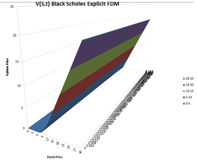
The orientation has been adjusted so that the solution curve at $t=0$ is clearly visible (the one of interest).

Exact pricing formula for a binary put or call

Consider a contract that pays $B=1$ if $S(T)\geq K$ at the terminal time $T$ (and $B=0$ if $S(T)<K$), where $S$ follows the geometric brownian motion process

$$S(t)-S_{0}=\mu\int_{0}^{t}S(t)\;dt+\sigma\int_{0}^{t}S(t)\;dW(t).$$

In "differential" form,

$$dS_{t}=\mu S_{t}dt+\sigma S_{t}dW_{t}.$$

This contract is known as a binary call option.  We seek to determine its price $V$ at the initial time $t=0$.  

The Black-Scholes theory implies (through its connection to parabolic partial differential equations and the Feyman-Kac formula) that this price is equal to the risk-neutral expected payoff $\mathbb{E}_{\mathbb{Q}}$ discounted at the risk-free rate $r$.  That is,

$$V=e^{-rT}\mathbb{E}_{\mathbb{Q}}[B].$$

A simple computation reveals that this is equal to $e^{-rT}\mathbb{Q}(S_{T}>K)$.  In detail,

$$e^{rT}V=\mathbb{E}_{\mathbb{Q}}[B]=1\cdot\mathbb{Q}(B=1)+0\cdot\mathbb{Q}(B=0)=\mathbb{Q}(B=1)=\mathbb{Q}(S_{T}>K).$$

Now, as covered in the Black-Scholes theory, an application of Girsonov's theorem leads us to the equivalent process for $S$
$$dS=rSdt+\sigma Sd\tilde{W_{t}}$$
where $\tilde{W}$ is a Brownian motion under the equivalent martingale measure (risk-neutral measure) $\mathbb{Q}$.  We now proceed as usual taking the natural logarithm to get
$$d\log S=(r-\frac{1}{2}\sigma^{2})dt+\sigma d\tilde{W_{t}},$$
which, in light of the risk-neutral probability computation above, immediately leads us to
$$\mathbb{E}_{\mathbb{Q}}[B]=N(d_{2}),$$
where $N=\Phi(0,1)$, the standard normal density, and
$$d_{2}=\frac{\ln(S_{0}/K)+(r-\frac{1}{2}\sigma^{2})T}{\sigma\sqrt{T}}.$$
Thus,
$$V=e^{-rT}N(d_{2}).$$
The price of the put can be determined by following the steps above, but where the contract has a payoff of $1$ when $S(T)\leq K$.  The result is
$$V=e^{-rT}N(d_{1}),$$
or equivalently
$$V=e^{-rt}N(-d_{2}).$$

As an aside from this, we can compute the price of this option using only the known prices of European call options.  Observe that the payoff function $P$ of this option is given by
$$P=\frac{\partial C_{K}}{\partial S}$$
where $C$ is the payoff function for European call option with strike price $K$.
This observation leads us to the conclusion
$$V=\lim_{\delta\to0}\frac{{U(K-\delta})-U(K)}{\delta}=-\frac{\partial U}{\partial S},$$
where $U(K)$ is the value of the call option with strike $K$.