Explicit Finite Difference Method for Black-Scholes-Merton PDE (European Calls)

Here we will implement a basic finite difference method to the solution of the Black-Scholes-Merton PDE
$$(1)\;\;\;\;\frac{\partial V}{\partial t}+\frac{1}{2}\sigma^{2}S^{2}\frac{\partial^{2}V}{\partial S^{2}}+rS\frac{\partial V}{\partial S}-rV=0,$$
which of course models the value $V$ of any derivative contract in the absence of arbitrage (see the Wikipedia article for a more comprehensive list of assumptions under which the Black-Scholes-Merton model is valid).

This PDE is a backwards diffusion (parabolic) equation: it is ill-posed in forward time.  This means that "initial conditions" are prescribed at $t=T$, the expiry time of the derivative being priced (in the case of this article, an option).  This is analogous to the prototypical heat equation $u_{t}=\Delta u,$ which is ill-posed in backward time, and hence requires initial conditions to be prescribed at time $t=0$.  It makes sense that a reverse-time evolution equation would model the value of a derivative since the payoff of the conract is known at the time of expiry $t=T$, and it is at the initial time $t=0$ that we are interested in knowing the "correct" value of the contract.  Indeed, we assume that the underlying of the derivative is a stock which follows a geometric Browning motion $\{S_{t}\}_{t\geq0}$ as in the Black-Scholes-Merton model.  This is a stochastic process for which we know $S_{0}$ (the time that the contract is being sold) and so the Black-Scholes equation allows us to compute $V(S(t),t)\big|_{t=0}=V(S_{0},0)$, which is the value of the contract today with observed stock price $S_{0}$.

The above discussion gives us an indication as to what boundary conditions must be prescribed in order that the solution $V(S,t)$ corresponds to the particular derivative contract being valued.  Indeed, (1) gives the value of any derivative; it is the boundary conditions which specify which derivative.  We shall consider the PDE to be defined on the $(S,t)$ space $[0,\bar{S}]\times[0,T]$ where $\bar{S}$ is the maximal stock price (typically $\bar{S}$ is taken to be $\bar{S}\approx 3K$, where $K$ is the strike price of the option).  (Ideally, we would have $\bar{S}=\infty$ so that we could apply the natural bounary condition $V(S,t)\to S$ as $S\to\infty$, but we must use a finite domain when applying finite differences.)  We then have the following boundary-value problem corresponding to (1)

$$\left\{\begin{array}{ll}
\frac{\partial V}{\partial t}+\frac{1}{2}\sigma^{2}S^{2}\frac{\partial^{2}V}{\partial S^{2}}+rS\frac{\partial V}{\partial S}-rV=0,&0\leq t< T, 0<S<\bar{S}\\
V(S,T)=\max(S-K,0),&t=T\\
V(0,t)=0,&S=0\\
V(\bar{S},t)=\bar{S}-Ke^{-r(T-t)},&S=\bar{S}.\end{array}\right.
$$

We now discretize the domain into increments $\Delta S$ and $\Delta t$.  The following notation is used: $k=\Delta t$, $h=\Delta S,$ $V_{m}^{n}=V(mh, nk),$ $N=T/k$, $M=\bar{S}/h.$  For simplicity we start with forward differences in time and centered differences in space to get (after some algebra)
$$V_{m}^{n}=A_{m}V_{m-1}^{n+1}+B_{m}V_{m}^{n+1}+C_{m}V_{m+1}^{n+1}$$
where
$$\begin{array}{l}
A_{m}=\frac{k}{2}\left(\sigma^{2}m^{2}-rm\right)\\
B_{m}=(1-k)(r\sigma^{2}m^{2})\\
C_{m}=\frac{k}{2}\left(\sigma^{2}m^{2}+rm\right)\end{array}
$$

Recall that the evolution is backward in time, so that this method is indeed explicit.

The following method was coded in Excel VBA using the method discussed above.  In this implementation we have used parameters $T=0.25$ (expiry in 3 months), $K=10$ (strike price 10 USD), $r=0.1$ and $\sigma=0.4.$

BS_FDM_Explicit.xlsm (Coded in Excel VBA)

Sub BSFiniteDifferenceScheme()

    ' User defined parameters
    Dim Riskless As Double
    Dim Vol As Double
    Dim Expiry As Double
    Dim Strike As Double
    
    Riskless = 0.1
    Vol = 0.4
    Expiry = 0.25
    Strike = 10
    
    ' Finite difference parameters
    Dim T As Double ' final time
    Dim S As Double ' stock price upper limit
    Dim N As Integer ' temporal steps
    Dim M As Integer ' stock steps
    Dim k As Double ' time step
    Dim h As Double ' stock step
    Dim V() As Double ' solution V(s,t)
    Dim T_Array() As Double
    Dim S_Array() As Double
    
    ' Set preliminary parameters
    T = Expiry
    S = 30
    k = 0.001
    h = 0.5
    N = T / k
    M = S / h
    ReDim V(N, M)
    
    For i = N To 0 Step -1
        Cells(i + 2, 1) = i * k
    Next i
    For j = 0 To M
        Cells(1, j + 2) = j * h
    Next j
    
    ' Set left boundary condition (S=0)
    For i = N To 0 Step -1
        V(i, 0) = 0
        Cells(i + 2, 2) = V(i, 0)
    Next i
    
    ' Set upper boundary condition (t=T)
    For j = 0 To M
        If j * h > Strike Then
            V(N, j) = j * h - Strike
        Else
            V(N, j) = 0
        End If
        Cells(N + 2, j + 2) = V(N, j)
    Next j
    
    ' Set right boundary condition (S=S_max)
    For i = N To 0 Step -1
        V(i, M) = S - Strike * Exp(-Riskless * (T - i * k))
        'V(i, M) = S
        Cells(i + 2, M + 2) = V(i, M)
    Next i
    
    ' Computation Loop
    Dim A As Double
    Dim B As Double
    Dim C As Double
    For i = N - 1 To 0 Step -1
        For j = 1 To M - 1
            A = (k / 2) * (Vol ^ 2 * j ^ 2 - Riskless * j)
            B = 1 - k * (Riskless + Vol ^ 2 * j ^ 2)
            C = (k / 2) * (Vol ^ 2 * j ^ 2 + Riskless * j)
            V(i, j) = A * V(i + 1, j - 1) + B * V(i + 1, j) + C * V(i + 1, j + 1)
            Cells(i + 2, j + 2) = V(i, j)
        Next j
    Next i
   
End Sub

The output has been setup to give the value of $V(S,t)$ for any pair $(S,t)$.  The table of data is of course to large to be given here, and of course we are only interested in the data $V(S_{0},0)$ where $S_{0}$ is the spot price at $t=0$.  For example, when $S_{0}=20$ the computation gives $V(20,0)=10.25$ USD.  This is the price at time $t=0$ for the option to buy a stock at time $T=0.25$ years when the current spot price is $20$ USD and the strike price is $10$ USD.  This rather high price (relative to the stock price) makes sense considering that the option is deep in the money and likely to be exercised at expiry.  To check that our value is indeed correct, we run the Monte Carlo simulation discussed in this post with identical parameters; the computed value with $N=10000$ trials is $V=10.21$ USD.  If we increase $N$ to $N=1000000$ (one million), we get with much greater consistency $V=10.25$, which is in agreement with our finite difference computation.

A graph produced from the output in Excel is given below.

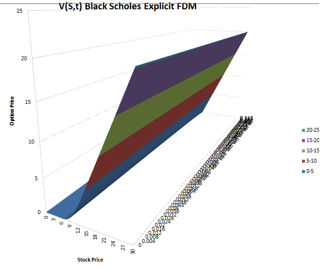
The orientation has been adjusted so that the solution curve at $t=0$ is clearly visible (the one of interest).

Exact pricing formula for a binary put or call

Consider a contract that pays $B=1$ if $S(T)\geq K$ at the terminal time $T$ (and $B=0$ if $S(T)<K$), where $S$ follows the geometric brownian motion process

$$S(t)-S_{0}=\mu\int_{0}^{t}S(t)\;dt+\sigma\int_{0}^{t}S(t)\;dW(t).$$

In "differential" form,

$$dS_{t}=\mu S_{t}dt+\sigma S_{t}dW_{t}.$$

This contract is known as a binary call option.  We seek to determine its price $V$ at the initial time $t=0$.  

The Black-Scholes theory implies (through its connection to parabolic partial differential equations and the Feyman-Kac formula) that this price is equal to the risk-neutral expected payoff $\mathbb{E}_{\mathbb{Q}}$ discounted at the risk-free rate $r$.  That is,

$$V=e^{-rT}\mathbb{E}_{\mathbb{Q}}[B].$$

A simple computation reveals that this is equal to $e^{-rT}\mathbb{Q}(S_{T}>K)$.  In detail,

$$e^{rT}V=\mathbb{E}_{\mathbb{Q}}[B]=1\cdot\mathbb{Q}(B=1)+0\cdot\mathbb{Q}(B=0)=\mathbb{Q}(B=1)=\mathbb{Q}(S_{T}>K).$$

Now, as covered in the Black-Scholes theory, an application of Girsonov's theorem leads us to the equivalent process for $S$
$$dS=rSdt+\sigma Sd\tilde{W_{t}}$$
where $\tilde{W}$ is a Brownian motion under the equivalent martingale measure (risk-neutral measure) $\mathbb{Q}$.  We now proceed as usual taking the natural logarithm to get
$$d\log S=(r-\frac{1}{2}\sigma^{2})dt+\sigma d\tilde{W_{t}},$$
which, in light of the risk-neutral probability computation above, immediately leads us to
$$\mathbb{E}_{\mathbb{Q}}[B]=N(d_{2}),$$
where $N=\Phi(0,1)$, the standard normal density, and
$$d_{2}=\frac{\ln(S_{0}/K)+(r-\frac{1}{2}\sigma^{2})T}{\sigma\sqrt{T}}.$$
Thus,
$$V=e^{-rT}N(d_{2}).$$
The price of the put can be determined by following the steps above, but where the contract has a payoff of $1$ when $S(T)\leq K$.  The result is
$$V=e^{-rT}N(d_{1}),$$
or equivalently
$$V=e^{-rt}N(-d_{2}).$$

As an aside from this, we can compute the price of this option using only the known prices of European call options.  Observe that the payoff function $P$ of this option is given by
$$P=\frac{\partial C_{K}}{\partial S}$$
where $C$ is the payoff function for European call option with strike price $K$.
This observation leads us to the conclusion
$$V=\lim_{\delta\to0}\frac{{U(K-\delta})-U(K)}{\delta}=-\frac{\partial U}{\partial S},$$
where $U(K)$ is the value of the call option with strike $K$.

Forward Spot Rate Curves

Consider a vector of maturities $(m_{1},\ldots,m_{N})$ and corresponding spot (zero) rate vector at time $t\geq0$ (which could be obtained from bootstrapping for instance, or in the case of LIBOR rates already given):
$$\left(S_{t}^{(m_{1})},\ldots,S_{t}^{(m_{N})}\right).$$
This can be viewed as a stochastic process with state space $\mathbb{R}^{N}$ or as $N$ individual stochastic processes $\{S^{(m_{j})}_{t}\}_{t\geq0}$ for $m_{j}\in\{m_{1},\ldots,m_{N}\}$ with state space $\mathbb{R}$.  Corresponding to this process is a forward process
$$\left\{\left(f_{t}^{(m_{1})}(T),\ldots,f_{t}^{(m_{N})}(T)\right)\right\}_{t\geq0}$$
that has an extra (deterministic) dimension in the variable $T$ and therefore the forward process has state space $\mathcal{C}(\mathbb{R})^{N}$.  Let us isolate our attention to one component of this process, say $f_{t}^{(m_{j})}(T)$ for some $1\leq j\leq N$, the forward spot rate process corresponding to maturity $m_{j}$ and future time $T$.  How do we determine this process in terms of $S^{m_{j}}_{t}$ so that for each $T\geq0$ the usual arbitrage conditions are satisfied?  For a non-dividend paying stock, the process is given by
$$f_{t}(T)=S_{t}e^{r(T-t)}.$$
But there is no obvious analogue for interest rates.  In fact, $f_{t}^{(m_{j})}(T)$ will depend on two components of the spot rate process for each $T$.  The definition is
$$(1)\;\;\;\;f^{(m_{j})}_{t}(T)=\frac{S^{(T+m_{j})}_{t}(T+m_{j})-S^{(T)}_{t}T}{m_{j}}.$$
This is obtained by equating the cash flows of borrowing at $S^{(T+m_{j})}_{t}$ for $T+m_{j}$ years versus borrowing at $S^{(T)}_{t}$ for $T$ years and then rolling forward the returns at $f^{(m_{j})}_{t}(T)$ for $m_{j}$ years.  This of course restricts $T$ to the set $\mathcal{T_{j}}:=\{m_{i}\}_{1\leq i\leq N-k(j)}$ where $k(j)$ is such that $T+m_{j}\leq m_{N}$ for all $T\in\mathcal{T_{j}}$.

An equivalent and more commonly encountered way to express this is to write
$$(2)\;\;\;\;f^{(m_{j})}_{t}(T_{1},T_{2})=\frac{S^{(T_{2})}_{t}T_{2}-S_{t}^{(T_{1})}T_{1}}{T_{2}-T_{1}}.$$
In this case, we require $T_{2}-T_{1}=m_{j}$ and $m_{1}\leq T_{2}\leq m_{N}.$  Of course, if we are interested in a forward rate at time $T$ that is not compatable with the spot rate vector that we have available at time $t$, then we can interpolate the pot curve (although this could potentially lead to arbitrage opportunities if you (a bank, say) are using this forward curve to price fixed income derivatives such as a swaps, because it is conceivable that a potential arbitrageur could get a spot rate for that interpolated term date different from your interpolated value!).

If we compute (1) for all $T\in\mathcal{T}_{j}$ we get a vector of points that represents the forward curve for the spot rate $S^{(m_{j})}_{t}$ associated with term $m_{j}$ computed at time $t$.  If we then do this for each $1\leq j\leq N$, we get a set of forward curves, one for each spot rate term.  If we fix a $T$ and plot $f^{(m_{j})}_{t}(T)$ for each $m_{j}$, then we get a forward term structure curve corresponding to the forward time $T$.  The particular interpretation taken depends on the context; usually the former is used for evaluating swap derivatives and the ladder for evaluating bond derivatives.

Valuing European FX (Currency) Options

I. Overview

A currency option is a contract that gives the buying party the right, but not the obligation, to buy (call) or sell (put) a foreign currency at a pre-defined exchange rate (strike).

For a given currency pair (e.g. EURJPY), the call or put designation of the option contract always refers to the base currency; therefore, the foreign currency is the base currency and the domestic currency is the quoted currency.  For example, a Japanese company expects to make a payment of 1,000,000 Euros in six months; they can hedge this exposure (while also participating in favorable price movements) by purchasing a call option on EUR/JPY.  Similarly, if they expected to receive Euros, they'd enter into a put option on EUR/JPY.

Because of the nature of FX transactions, every currency option is technically two options: a call and a put.  So a call on EUR/JPY is a call (buy/receive) on EUR and a put (sell/give) on JPY for a specified exchange rate (the strike) and a put on EUR/JPY is a put (sell/give) on EUR and a call (buy/receive) on JPY.

Exercise.  Sometimes a currency pair is not actively quoted.  For example, if the domestic currency is EUR and the foreign currency is JPY, the pair underlying a given currency contract would be JPY/EUR, which is not actively quoted.  Of course, one could simply invert this currency pair and the above discussion applies with this exchange rate.  However, show that for currencies C1 and C2 that a call (put) on C1/C2 is a equivalent to a put (call) on C2/C1.  So if the European company (domestic currency) wants to buy a put on JPY/EUR (they want to sell JPY that they expect to receive sometime in the future for EUR), then they can buy an (equivalent) call on EUR/JPY.

As a final note, each currency has an associated risk free rate $r_{d}$ and $r_{f}$ (domestic and floating, respectively). 

 II. Valuation Theory

The Black-Scholes model on a dividend paying equity is easily adapted to the present situation by regarding the currency pair exchange rate as a price with an associated volatility and the foreign riskless rate as a dividend yield.  The justification for the ladder follows the same cost of carry argument as in the case of a dividend.

The usual formulas are
$$c(S,t)=Se^{-r_{f}(T-t)}\mathbb{N}(d_{1})-Ke^{-r_{d}(T-t)}\mathbb{N}(d_{2})$$
and
$$p(S,t)=Ke^{-r_{d}(T-t)}\mathbb{N}(-d_{2})-Se^{-r_{f}(T-t)}\mathbb{N}(-d_{1})$$
where of course
$$d_{1}=\frac{\log(S/K)+(r_{d}-r_{f}+\sigma^{2}/2)(T-t)}{\sigma\sqrt{T-t}}$$
and
$$d_{2}=d_{1}-\sigma\sqrt{T-t}.$$

Because $F_{t}=S_{t}e^{-(r_{d}r_{f})(T-t)}$, the forward price of the currency pair, the formulas above can be simplified to

Thus one only needs the discount rate in the domestic currency.

III. Example

Consider a call on

Analysis of Pricing European Options

I. INTRODUCTION

This post begins a eight part series of posts having to do with the analysis and practical implementation of options pricing including European options, American options, Asian options (and other options with path-dependent payoffs), and other exotic options not covered in previous posts (barriers, knock-outs, etc.).

The analysis of European option pricing is by far the most complete in the sense that one can obtain useful no-arbitrage bounds without appealing to any underlying asset price evolution model and even an exact relationship known as put-call parity.  Furthermore, exact pricing formulas when geometric Brownian motion is assumed for asset price evolution can be achieved.

II. NO ARBITRAGE BOUNDS

While it is possible to obtain exact pricing formulas for European options, it is instructive to first see what can be accomplished by consider no-arbitrage arguments.  This is so for two principle reasons: one, the arguments do not require us to assume any particular asset price evolution model - the conclusions are valid in any complete market that does not permit arbitrage - and two, the arguments lead to easy to remember bounds on European option prices that are useful to keep in mind as a sanity check for when one is numerically computing prices; furthermore, when certain parameters approach extreme values, the bounds obtained tend to become sharp and approximately agree with each other, thus yielding the option's price (which is an even more legitimate price since, once again, no assumptions are made about how the underlying asset evolves in time).

Let us denote by $c(S,t)$ and $p(S,t)$ the values of European options at time $t$ where $S=S(t)$ is the underlying asset's price at time $t$.  We are primarily interested in determining $c:=c(S_{0},0)$ and $p:=(S_{0},0)$, the premium paid by the buyer for the right to exercise an option at a future time.  These quantities are of course non-trivial since options always have positive value at time $t=0$ (unless of course $S_{0}\equiv0$), and this is what makes pricing options significantly more difficult (and interesting) than the pricing of "zero-sum" derivatives like futures and swaps that have a value of $0$ and time $t=0$, and in any event are easily priced at all future times (we will not concern ourselves with the pricing of options at future times in this section, since as mentioned, it is much more important to know the values at the intial time $t=0$).

Suppose that we sell a put option for $p$ dollars and invest the proceeds into the risk-free money market account so that at expiry we have $pe^{rT}$ dollars.  If $S_{T}\geq K$ then the option is worthless and we have $pe^{rT}$ dollars.  If $S_{T}<K$, then the buyer will exercise the put option and we then have $pe^{rT}-K$ dollars.  If $p>Ke^{-rT}$, then in both cases we have made a riskless profit of at least $pe^{rT}-K>0$ from a portfolio that cost nothing to setup.  This arbitrage opportunity is only possible if $p>Ke^{-rT}$.  This yields the no-arbitrage upper bound

$$p\leq Ke^{-rT}.$$

Similarly, if we sell a call option for $c$ dollars and cover our obligation to sell the underlying asset for $K$ dollars by buying the asset today for $S_{0}$ dollars, then we can make a riskless profit from a portfolio that cost nothing to setup if and only if $c>S_{0}$.  Thus,

$$c\leq S_{0}.$$

(It is instructive to think about why the upper bound for $p$ involves $K$ and discounting while the upper bound for $c$ involves $S_{0}$ and no discounting, and that there is no alternative to this which is sharper.)

To obtain a lower bound, suppose that ...

III. PUT-CALL PARTIY

It is a rather remarkable fact that there exists a function $\Phi$ such that $\Phi(c,p)=0$.  This fact is known as put-call parity and it allows on to price $p$ given $c$ and vice versa, with only the assumption of no-arbitrage.

To derive it, consider a portfolio $A$ consisting of ... and a portfolio $B$ consisting of ...

IV.  EXACT PRICING FORMULAS

If we move from our realistic no-arbitrage world to that of Black-Scholes, we can obtain exact pricing formulas for $c$ and $p$ (for all times $0\leq t\leq T$ too!).  The Black-Scholes model is discussed in this previous post ... The main quantitative assumption (in addition to the various qualitative market assumptions) is that the underlying asset follows the geometric Brownian motion process

$$S(t)=S(0)+\int_{0}^{t}\mu S(\tau)\;d\tau+\int_{0}^{t}\sigma S(\tau)\;dW(\tau),$$

where $\{W_{t}\}_{t\geq0}$ is a Brownian motion.  Under this assumption, we derived the PDE

$$V_{t}+\frac{1}{2}\sigma^{2}S^{2}V_{SS}+rSV_{S}-rV=0,$$

for which any derivative depending on $S$ must satisfy (i.e. $c=c(S,t)$ and $p=p(S,t)$ must satisfy the PDE).  By solving this PDE with boundary and terminal conditions characteristic of the particular derivative under consideration, we get a deterministic pricing function $V$ for the derivative, valid for all time $t\geq0$ and asset price paths $\{S_{t}\}_{t\geq0}$.

Basic financial considerations derived from the previous sections lead to the following BVP for $c$:

\[\left\{\begin{array}{rr}c_{t}+\frac{1}{2}\sigma^{2}S^{2}c_{SS}+rSc_{S}-rc=0,&(S,t)\in(0,\infty)\times(0,T)\\c(S,T)=\max(S-K,0)&\\c(0,t)=0&.\\\lim_{S\to\infty}c(S,t)=S&\end{array}\right.\]

(It should be understood that while $S=S(t)$ so that $c=c(S(t),t)=c(t)$, we generally consider $c$ to be a function two variables $(S,t)$, particularly when working directly with the PDE so that for instance the terminal condition is written as above instead of as $c(S(T),T)=\max(S(T)-K,0)$.)

Similarly, for $p$ we have the BVP:

\[\left\{\begin{array}{rr}p_{t}+\frac{1}{2}\sigma^{2}S^{2}p_{SS}+rSp_{S}-rp=0,&(S,t)\in(0,\infty)\times(0,T)\\p(S,T)=\max(K-S,0)&\\p(0,t)=Ke^{-r(T-t)}&.\\\lim_{S\to\infty}c(S,t)=0&\end{array}\right.\]

Let us solve the BVP for $c$.  In this previous post on the analysis of the PDE, we discussed how to transform the Black-Scholes PDE into the heat equation by making a succession of variable changes in order to eliminate the various lower order terms.  Review that post to see the transformation carried out in detail; here we just summarize the order of the transformations to be carried out and the resulting BVP: