
$$(1)\;\;\;\;\frac{\partial V}{\partial t}+\frac{1}{2}\sigma^{2}S^{2}\frac{\partial^{2}V}{\partial S^{2}}+rS\frac{\partial V}{\partial S}-rV=0,$$
which of course models the value $V$ of any derivative contract in the absence of arbitrage (see the Wikipedia article for a more comprehensive list of assumptions under which the Black-Scholes-Merton model is valid).
This PDE is a backwards diffusion (parabolic) equation: it is ill-posed in forward time. This means that "initial conditions" are prescribed at $t=T$, the expiry time of the derivative being priced (in the case of this article, an option). This is analogous to the prototypical heat equation $u_{t}=\Delta u,$ which is ill-posed in backward time, and hence requires initial conditions to be prescribed at time $t=0$. It makes sense that a reverse-time evolution equation would model the value of a derivative since the payoff of the conract is known at the time of expiry $t=T$, and it is at the initial time $t=0$ that we are interested in knowing the "correct" value of the contract. Indeed, we assume that the underlying of the derivative is a stock which follows a geometric Browning motion $\{S_{t}\}_{t\geq0}$ as in the Black-Scholes-Merton model. This is a stochastic process for which we know $S_{0}$ (the time that the contract is being sold) and so the Black-Scholes equation allows us to compute $V(S(t),t)\big|_{t=0}=V(S_{0},0)$, which is the value of the contract today with observed stock price $S_{0}$.
The above discussion gives us an indication as to what boundary conditions must be prescribed in order that the solution $V(S,t)$ corresponds to the particular derivative contract being valued. Indeed, (1) gives the value of any derivative; it is the boundary conditions which specify which derivative. We shall consider the PDE to be defined on the $(S,t)$ space $[0,\bar{S}]\times[0,T]$ where $\bar{S}$ is the maximal stock price (typically $\bar{S}$ is taken to be $\bar{S}\approx 3K$, where $K$ is the strike price of the option). (Ideally, we would have $\bar{S}=\infty$ so that we could apply the natural bounary condition $V(S,t)\to S$ as $S\to\infty$, but we must use a finite domain when applying finite differences.) We then have the following boundary-value problem corresponding to (1)
$$\left\{\begin{array}{ll}
\frac{\partial V}{\partial t}+\frac{1}{2}\sigma^{2}S^{2}\frac{\partial^{2}V}{\partial S^{2}}+rS\frac{\partial V}{\partial S}-rV=0,&0\leq t< T, 0<S<\bar{S}\\
V(S,T)=\max(S-K,0),&t=T\\
V(0,t)=0,&S=0\\
V(\bar{S},t)=\bar{S}-Ke^{-r(T-t)},&S=\bar{S}.\end{array}\right.
$$
We now discretize the domain into increments $\Delta S$ and $\Delta t$. The following notation is used: $k=\Delta t$, $h=\Delta S,$ $V_{m}^{n}=V(mh, nk),$ $N=T/k$, $M=\bar{S}/h.$ For simplicity we start with forward differences in time and centered differences in space to get (after some algebra)
$$V_{m}^{n}=A_{m}V_{m-1}^{n+1}+B_{m}V_{m}^{n+1}+C_{m}V_{m+1}^{n+1}$$
where
$$\begin{array}{l}
A_{m}=\frac{k}{2}\left(\sigma^{2}m^{2}-rm\right)\\
B_{m}=(1-k)(r\sigma^{2}m^{2})\\
C_{m}=\frac{k}{2}\left(\sigma^{2}m^{2}+rm\right)\end{array}
$$
Recall that the evolution is backward in time, so that this method is indeed explicit.
The following method was coded in Excel VBA using the method discussed above. In this implementation we have used parameters $T=0.25$ (expiry in 3 months), $K=10$ (strike price 10 USD), $r=0.1$ and $\sigma=0.4.$
BS_FDM_Explicit.xlsm (Coded in Excel VBA)
Sub BSFiniteDifferenceScheme()

    ' User defined parameters
    Dim Riskless As Double
    Dim Vol As Double
    Dim Expiry As Double
    Dim Strike As Double

    Riskless = 0.1
    Vol = 0.4
    Expiry = 0.25
    Strike = 10

    ' Finite difference parameters
    Dim T As Double ' final time
    Dim S As Double ' stock price upper limit
    Dim N As Integer ' temporal steps
    Dim M As Integer ' stock steps
    Dim k As Double ' time step
    Dim h As Double ' stock step
    Dim V() As Double ' solution V(s,t)
    Dim T_Array() As Double
    Dim S_Array() As Double

    ' Set preliminary parameters
    T = Expiry
    S = 30
    k = 0.001
    h = 0.5
    N = T / k
    M = S / h
    ReDim V(N, M)

    For i = N To 0 Step -1
        Cells(i + 2, 1) = i * k
    Next i
    For j = 0 To M
        Cells(1, j + 2) = j * h
    Next j

    ' Set left boundary condition (S=0)
    For i = N To 0 Step -1
        V(i, 0) = 0
        Cells(i + 2, 2) = V(i, 0)
    Next i

    ' Set upper boundary condition (t=T)
    For j = 0 To M
        If j * h > Strike Then
            V(N, j) = j * h - Strike
        Else
            V(N, j) = 0
        End If
        Cells(N + 2, j + 2) = V(N, j)
    Next j

    ' Set right boundary condition (S=S_max)
    For i = N To 0 Step -1
        V(i, M) = S - Strike * Exp(-Riskless * (T - i * k))
        'V(i, M) = S
        Cells(i + 2, M + 2) = V(i, M)
    Next i

    ' Computation Loop
    Dim A As Double
    Dim B As Double
    Dim C As Double
    For i = N - 1 To 0 Step -1
        For j = 1 To M - 1
            A = (k / 2) * (Vol ^ 2 * j ^ 2 - Riskless * j)
            B = 1 - k * (Riskless + Vol ^ 2 * j ^ 2)
            C = (k / 2) * (Vol ^ 2 * j ^ 2 + Riskless * j)
            V(i, j) = A * V(i + 1, j - 1) + B * V(i + 1, j) + C * V(i + 1, j + 1)
            Cells(i + 2, j + 2) = V(i, j)
        Next j
    Next i

End Sub
The output has been setup to give the value of $V(S,t)$ for any pair $(S,t)$. The table of data is of course to large to be given here, and of course we are only interested in the data $V(S_{0},0)$ where $S_{0}$ is the spot price at $t=0$. For example, when $S_{0}=20$ the computation gives $V(20,0)=10.25$ USD. This is the price at time $t=0$ for the option to buy a stock at time $T=0.25$ years when the current spot price is $20$ USD and the strike price is $10$ USD. This rather high price (relative to the stock price) makes sense considering that the option is deep in the money and likely to be exercised at expiry. To check that our value is indeed correct, we run the Monte Carlo simulation discussed in this post with identical parameters; the computed value with $N=10000$ trials is $V=10.21$ USD. If we increase $N$ to $N=1000000$ (one million), we get with much greater consistency $V=10.25$, which is in agreement with our finite difference computation.
A graph produced from the output in Excel is given below.
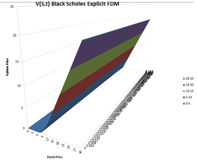
The orientation has been adjusted so that the solution curve at $t=0$ is clearly visible (the one of interest).